Quick Summary: Predictive analytics in Python leverages machine learning libraries like scikit-learn, XGBoost, and H2O to forecast future outcomes from historical data. Python’s ecosystem offers accessible tools for building, validating, and deploying predictive models across industries—from finance to healthcare—with frameworks that handle everything from data preprocessing to model evaluation.
Predictive analytics transforms raw data into actionable forecasts. It’s the practice of extracting patterns from historical datasets to predict future events—whether that’s customer churn, equipment failure, or market trends.
Python dominates this space for good reasons. The language combines approachable syntax with powerful libraries designed specifically for statistical modeling and machine learning. Developers and analysts alike can move from data exploration to production-grade predictions without switching tools.
Here’s the thing though—building effective predictive models requires more than just plugging data into algorithms. It demands understanding of model selection, validation techniques, and evaluation metrics that determine whether predictions actually hold up in the real world.
What Makes Predictive Analytics Different
Predictive analysis goes beyond describing what happened. Traditional analytics tells you that sales dropped last quarter. Predictive analytics estimates the probability they’ll drop next quarter and identifies which factors contribute most to that risk.
The approach utilizes statistical algorithms and machine learning techniques to identify likelihood of future outcomes based on historical data. It’s fundamentally about pattern recognition—training models to spot relationships between variables that human analysis might miss.
Industries apply these techniques differently. Financial institutions use predictive models to assess credit risk and detect fraud. Healthcare organizations predict patient readmission rates. Manufacturing plants forecast equipment maintenance needs before breakdowns occur.
Python’s ecosystem supports all these scenarios through specialized libraries. scikit-learn provides the foundational algorithms. XGBoost and H2O deliver advanced gradient boosting with distributed computing capabilities. Yellowbrick adds visual diagnostics for model selection and evaluation.

Use Predictive Analytics in Python with AI Superior
AI Superior builds predictive models using Python-based tools and libraries, focusing on real data and production-ready systems. They handle the full process from data assessment to model development and integration into existing infrastructure.
Looking to Build Predictive Models in Python?
AI Superior can help with:
- evaluating and preparing data
- building predictive models in Python
- integrating models into existing systems
- refining performance over time
👉 Contact AI Superior to discuss your project, data, and implementation approach.
Essential Python Libraries for Predictive Modeling
The Python data science stack builds on several core libraries that work together seamlessly.
- NumPy and Pandas handle data structures and manipulation. NumPy provides efficient array operations, while Pandas offers DataFrames for structured data analysis. Most predictive workflows start here—loading datasets, cleaning missing values, encoding categorical variables.
- scikit-learn serves as the workhorse for machine learning. It implements dozens of algorithms through a consistent API. The library includes tools for preprocessing, model selection, and evaluation metrics. Cross-validation utilities help assess how models generalize to new data.
- XGBoost implements extreme gradient boosting, a technique that often dominates predictive competitions. Research shows XGBoost achieves strong performance across classification tasks. In comparative analysis of default prediction, XGBoost demonstrated competitive metrics on binary classification problems.
- H2O brings distributed machine learning to Python. The library scales to large datasets through in-memory processing. The H2O package (version 3.46.0.10) is actively maintained on PyPI as of March 12, 2026, for fast, scalable machine learning applications.
- Yellowbrick extends scikit-learn with visualization tools specifically designed for model evaluation. Released August 21, 2022 (version 1.5, 20.0 MB), Yellowbrick provides visual diagnostics that help identify overfitting, feature importance, and classification performance at a glance.
Building Predictive Models Step-by-Step
Real-world predictive projects follow a consistent workflow regardless of the specific problem domain.
Data Collection and Preparation
Quality predictions require quality data. The first step involves gathering historical records that contain both the features (input variables) and the target (what needs prediction).
Data rarely arrives clean. Missing values need handling—either through imputation, removal, or indicator variables that flag missingness as potentially meaningful. Outliers require investigation. Are they data entry errors or legitimate extreme cases?
Categorical variables must be encoded numerically. One-hot encoding creates binary columns for each category. Label encoding assigns integers, which works for ordinal data but can mislead algorithms into seeing non-existent numeric relationships.
Feature scaling normalizes numeric ranges. Many algorithms perform better when all features share similar scales. StandardScaler transforms features to have zero mean and unit variance. MinMaxScaler compresses values into a fixed range, typically 0 to 1.
Train-Test Split and Cross-Validation
Testing a model on the same data used for training guarantees overfitting. The model memorizes specific examples rather than learning generalizable patterns.
The solution splits data into training and test sets. scikit-learn provides train_test_split for this purpose. Common splits allocate 70-80% for training and reserve 20-30% for final evaluation.
But here’s the problem—a single train-test split can be misleading. Maybe the test set happened to be unusually easy or hard. Cross-validation addresses this by splitting data multiple ways and averaging results.
K-fold cross-validation divides data into K equal parts. The model trains on K-1 parts and tests on the remaining part, rotating through all combinations. Five or ten folds balance computational cost with reliable estimates of model performance.
Algorithm Selection
Different algorithms suit different prediction tasks. The choice depends on the target variable type, dataset size, interpretability requirements, and performance constraints.
- Logistic Regression works for binary or multi-class classification when relationships between features and outcomes are roughly linear. It’s fast, interpretable, and serves as a strong baseline. Research on credit default prediction found logistic regression achieved 0.7679 AUC with 0.63 recall (0.58-0.69 CI) in comparative testing.
- Decision Trees split data recursively based on feature values. They handle non-linear relationships naturally and require minimal preprocessing. Comparative analysis showed decision trees reaching 0.80 AUC with 0.63 recall (0.58-0.68 CI) and 0.63 precision (0.58-0.68 CI), though they tend to overfit without pruning.
- Random Forests combine multiple decision trees to reduce overfitting. Each tree trains on a random subset of data and features. Predictions aggregate across all trees. Performance metrics from classification studies show Random Forest achieving 0.98 AUC with 0.77 recall (0.72-0.81 CI), 0.96 precision (0.94-0.98 CI), and 0.85 F1-score (0.81-0.89 CI).
- Gradient Boosting builds trees sequentially, with each new tree correcting errors from previous ones. The technique achieves high accuracy at the cost of longer training times. Comparative analysis demonstrates Gradient Boosting models reaching 0.92 AUC with 0.80 recall (0.76-0.84 CI), 0.80 precision (0.76-0.84 CI), and 0.80 F1-score (0.76-0.84 CI).
- XGBoost optimizes gradient boosting with regularization and parallel processing. It handles missing values internally and provides feature importance scores. The algorithm consistently performs well—testing shows 0.94 AUC with 0.77 recall (0.72-0.81 CI), 1.0 precision, and 0.87 F1-score (0.83-0.90 CI) when tuned properly.
| Algorithm | AUC | Recall | Precision | F1-Score |
|---|---|---|---|---|
| Random Forest | 0.98 | 0.77 (0.72-0.81) | 0.96 (0.94-0.98) | 0.85 (0.81-0.89) |
| XGBoost | 0.94 | 0.77 (0.72-0.81) | 1.0 (1-1) | 0.87 (0.83-0.90) |
| Gradient Boosting | 0.92 | 0.80 (0.76-0.84) | 0.80 (0.76-0.84) | 0.80 (0.76-0.84) |
| Decision Tree | 0.80 | 0.63 (0.58-0.68) | 0.63 (0.58-0.68) | — |
| Logistic Regression | 0.7679 | 0.63 (0.58-0.69) | — | — |
Model Training and Hyperparameter Tuning
Training fits the algorithm to data, adjusting internal parameters to minimize prediction error. scikit-learn uses a consistent fit() method across all estimators.
Hyperparameters control how the algorithm learns but aren’t learned from data themselves. Random Forest needs the number of trees and maximum tree depth specified. XGBoost requires learning rate, max depth, and regularization terms.
Grid search tests every combination of specified hyperparameter values. It’s thorough but computationally expensive. Randomized search samples combinations randomly, covering more parameter space with fewer iterations.
Successive halving allocates resources efficiently by quickly eliminating poor hyperparameter combinations and focusing compute time on promising candidates.
Model Evaluation Metrics
Accuracy—the percentage of correct predictions—seems intuitive but can be misleading. A model predicting “no fraud” for every transaction achieves 99% accuracy if fraud occurs in just 1% of cases, yet it’s completely useless for fraud detection.
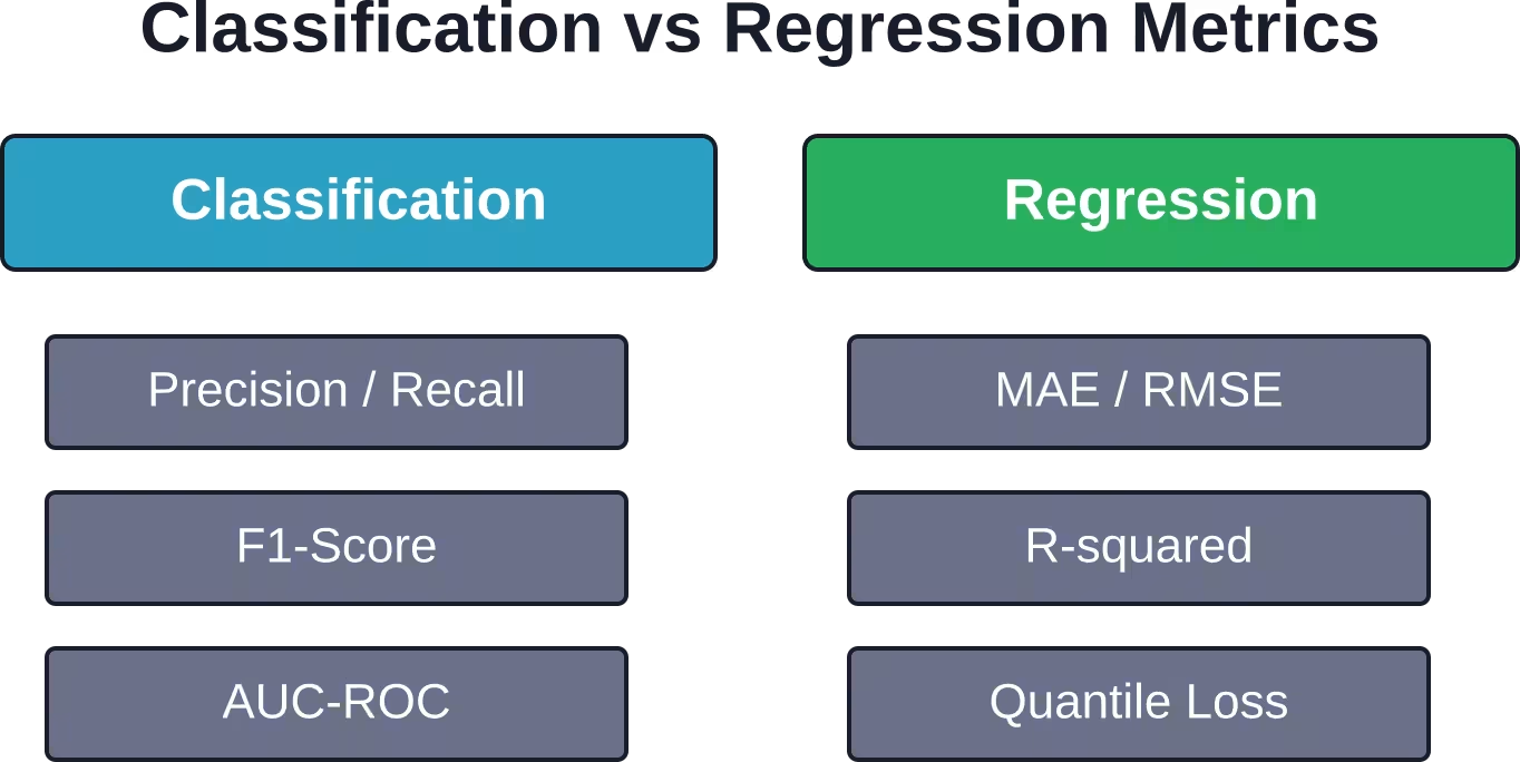
Classification Metrics
- Precision measures how many positive predictions were actually correct. High precision means few false alarms. Financial fraud detection prioritizes precision to avoid blocking legitimate transactions.
- Recall (also called sensitivity) measures how many actual positives the model caught. Medical screening prioritizes recall—missing a disease diagnosis has serious consequences even if it means more false positives.
- F1-Score combines precision and recall into a single metric through their harmonic mean. It balances both concerns and works well when class distribution is imbalanced.
- AUC-ROC (Area Under the Receiver Operating Characteristic curve) measures how well the model separates classes across all possible classification thresholds. Values near 1.0 indicate excellent separation. The metric works regardless of class imbalance.
- Log Loss quantifies prediction confidence. It penalizes confident wrong predictions more heavily than uncertain ones. For a probability prediction example with predict_proba on binary classification, scikit-learn documentation shows a log loss value of 0.1738 for sample predictions.
Regression Metrics
When predicting continuous values rather than categories, different metrics apply.
- Mean Absolute Error (MAE) averages the absolute differences between predictions and actual values. It’s interpretable in the original units and treats all errors equally.
- Root Mean Squared Error (RMSE) penalizes large errors more heavily by squaring differences before averaging. It’s more sensitive to outliers than MAE.
- R-squared measures the proportion of variance in the target explained by the model. Values range from 0 to 1, with higher values indicating better fit. But watch out—R-squared can be high even when predictions are systematically biased.
Practical Implementation Example
A complete predictive analytics workflow in Python typically looks like this:
| import pandas as pd from sklearn.model_selection import train_test_split from sklearn.preprocessing import StandardScaler from sklearn.ensemble import RandomForestClassifier from sklearn.metrics import classification_report, roc_auc_score # Load and prepare data df = pd.read_csv(‘data.csv’) X = df.drop(‘target’, axis=1) y = df[‘target’] # Split data X_train, X_test, y_train, y_test = train_test_split( X, y, test_size=0.2, random_state=42 ) # Scale features scaler = StandardScaler() X_train_scaled = scaler.fit_transform(X_train) X_test_scaled = scaler.transform(X_test) # Train model model = RandomForestClassifier( n_estimators=100, max_depth=10, random_state=42 ) model.fit(X_train_scaled, y_train) # Evaluate y_pred = model.predict(X_test_scaled) print(classification_report(y_test, y_pred)) print(‘AUC:’, roc_auc_score(y_test, model.predict_proba(X_test_scaled)[:, 1])) |
This pattern scales to more complex scenarios. The same structure applies whether working with hundreds of features or millions of records.
Feature Engineering
Raw data rarely provides the best predictive signal. Feature engineering creates new variables that make patterns more obvious to algorithms.
Time-based features extract components like day of week, month, or time since last event. These often correlate strongly with behavior patterns—retail sales vary by day, equipment failures cluster after certain usage durations.
Interaction features multiply or combine existing variables to capture relationships. Price times quantity gives total sale value. Temperature divided by humidity creates a derived climate metric.
Aggregation features summarize groups. Customer purchase frequency over the last 30 days, average transaction amount by merchant category, or standard deviation of sensor readings per machine.
Domain knowledge drives the best feature engineering. Subject matter experts recognize which combinations matter. A retail analyst knows seasonal purchasing patterns. A network engineer understands protocol interactions that signal anomalies.
Common Pitfalls and How to Avoid Them
Overfitting tops the list. Models that perform brilliantly on training data but fail on new data have memorized noise instead of learning patterns.
The warning signs include perfect or near-perfect training accuracy, large gaps between training and validation scores, and excessive model complexity (deep decision trees, hundreds of features, no regularization).
- Regularization techniques combat overfitting. L1 regularization (Lasso) shrinks some coefficients to zero, performing feature selection. L2 regularization (Ridge) penalizes large coefficients, encouraging simpler models. Early stopping in iterative algorithms halts training when validation performance stops improving.
- Data leakage occurs when information from the test set inadvertently influences training. This happens through several mechanisms.
- Scaling before splitting means test data statistics affect the scaler parameters. Always fit transformers on training data only, then apply the fitted transformer to test data.
- Target encoding categorical variables with the full dataset leaks target information. Compute encodings within cross-validation folds to maintain separation.
- Features that contain future information create artificial performance. A “days until churn” variable predicts churn perfectly but is calculated from the target—it would be unknown at prediction time.
- Imbalanced classes plague many real-world problems. Fraud detection, disease diagnosis, and equipment failure prediction all involve rare events.
- Resampling techniques adjust class distribution. SMOTE (Synthetic Minority Over-sampling Technique) generates synthetic examples of the minority class. Random undersampling removes majority class examples.
- Class weights tell algorithms to penalize minority class errors more heavily. Most scikit-learn classifiers accept a class_weight parameter that can be set to ‘balanced’ for automatic weighting.
- Evaluation metrics matter more than usual with imbalanced data. Precision, recall, and F1-score provide better signal than accuracy. Focus on the metric that aligns with business costs of false positives versus false negatives.
Advanced Techniques
Ensemble Methods
Combining predictions from multiple models often outperforms any single model. Different algorithms make different types of errors, and aggregating reduces individual model weaknesses.
Voting ensembles combine predictions through majority vote (classification) or averaging (regression). Train several diverse models—say Random Forest, XGBoost, and Logistic Regression—then aggregate their predictions.
Stacking trains a meta-model on predictions from base models. The base models generate predictions as features for the meta-model, which learns how to weight each base model’s contributions.
Time Series Forecasting
Temporal data requires special handling. Standard cross-validation randomly splits data, but past/future order matters for time series.
Time series cross-validation respects temporal order. Train on data up to time T, test on time T+1 to T+N, then roll forward and repeat. scikit-learn’s TimeSeriesSplit implements this pattern.
Feature engineering for time series includes lagged variables (values from T-1, T-2, etc.), rolling statistics (moving averages, exponential smoothing), and seasonal decomposition.
ARIMA and Prophet handle time series natively with seasonal and trend components. The statsmodels library provides ARIMA. Prophet, developed by Meta, handles missing data and outliers well while modeling complex seasonal patterns.
Model Interpretation
Understanding why a model makes specific predictions builds trust and enables improvement.
Feature importance scores rank variables by their contribution to predictions. Tree-based models calculate importance through split gain. Permutation importance measures performance drop when shuffling each feature.
SHAP (SHapley Additive exPlanations) values provide consistent feature attribution. They explain individual predictions by computing each feature’s contribution. The technique works across model types and satisfies desirable theoretical properties.
Partial dependence plots show how predictions change as a single feature varies while holding others constant. They reveal whether relationships are linear, monotonic, or complex.
Real-World Applications
Predictive analytics solves concrete business problems across every industry.
- Healthcare institutions predict patient readmission risk, enabling targeted intervention programs. Models identify which patients need follow-up appointments or home care support. Clinical diagnosis systems use predictive models to flag high-risk conditions earlier than traditional protocols.
- Finance relies heavily on predictive modeling for credit scoring, fraud detection, and algorithmic trading. Banks assess loan default probability before extending credit. Payment processors flag suspicious transactions in real-time. Investment firms forecast asset price movements and portfolio risk.
- Retail companies predict customer churn, lifetime value, and product demand. Recommendation engines suggest products based on purchase history and browsing behavior. Inventory optimization models forecast demand at the SKU and location level to minimize stockouts and overstock.
- Manufacturing implements predictive maintenance to reduce downtime. Sensors generate streams of data—temperature, vibration, pressure. Models learn failure patterns and predict when equipment needs service before breakdowns occur.
- Marketing teams use propensity models to identify which customers are most likely to respond to campaigns, make purchases, or engage with content. This targeting improves conversion rates and ROI by focusing resources on high-probability opportunities.
Model Deployment and Monitoring
A trained model provides no value until it generates predictions in production systems.
Deployment options range from batch scoring to real-time APIs. Batch processes generate predictions for all records on a schedule—nightly churn scores, weekly demand forecasts. REST APIs serve predictions on-demand when users or systems request them.
Flask and FastAPI provide lightweight frameworks for wrapping models in HTTP endpoints. The pattern loads the trained model file, accepts JSON input, runs preprocessing, generates predictions, and returns results.
Containerization through Docker ensures consistent environments across development, testing, and production. The container includes Python, required libraries, the model file, and serving code. Kubernetes orchestrates containers at scale with load balancing and automatic recovery.
Monitoring catches degradation before it causes problems. Log prediction distributions—if they shift dramatically from training data, the model may be seeing fundamentally different inputs.
Track performance metrics on labeled production data when available. If accuracy drops over time, the model needs retraining with fresh data. Drift in feature distributions signals that data patterns have changed.
Automated retraining pipelines keep models current. Schedule periodic retraining—monthly, quarterly, or when performance degrades past thresholds. Version control for models lets teams roll back if new versions underperform.
Resources for Learning More
The scikit-learn documentation provides comprehensive guidance on model selection, evaluation, and cross-validation. The library’s consistent API makes transitioning between algorithms straightforward.
Kaggle competitions offer hands-on practice with real datasets and community benchmarks. Working through past competitions exposes techniques used by top performers. Discussion forums explain solution approaches in detail.
Academic research archives like arXiv publish cutting-edge predictive analytics research. Comparative studies of machine learning algorithms provide performance baselines across problem domains. Research on specific applications—from potato variety prediction to credit scoring—demonstrates domain-specific techniques.
The H2O, XGBoost, and Yellowbrick package documentation on PyPI includes installation instructions, API references, and usage examples. These libraries extend beyond basic scikit-learn capabilities for specialized needs.
Online courses through platforms offering predictive analytics curricula cover everything from fundamentals to advanced topics. Look for courses that emphasize hands-on projects rather than just theory.
Frequently Asked Questions
What’s the difference between predictive analytics and machine learning?
Predictive analytics is the business application—using data to forecast outcomes. Machine learning is the technical approach—algorithms that learn patterns from data. Most modern predictive analytics relies on machine learning algorithms, but the terms emphasize different aspects of the same process.
How much data do I need for predictive modeling?
It depends on problem complexity and model type. Simple linear models work with hundreds of examples. Deep learning requires thousands or millions. A practical minimum is 10-20 examples per feature for basic models. Start with available data and assess whether performance meets requirements before investing in additional data collection.
Should I use Random Forest or XGBoost?
Both perform well for many tasks. Random Forest trains faster, requires less tuning, and rarely overfits badly. XGBoost often achieves slightly better accuracy with proper tuning but takes more computational resources. Start with Random Forest for baseline results, then try XGBoost if performance matters enough to justify the effort.
How do I handle imbalanced datasets?
Combine several approaches. Use appropriate evaluation metrics like F1-score instead of accuracy. Apply class weights to penalize minority class errors more heavily. Try resampling techniques like SMOTE to balance training data. Collect more examples of the minority class if possible. Ensemble different resampling strategies for robust predictions.
What’s the best way to prevent overfitting?
Cross-validation detects overfitting by testing on multiple held-out sets. Regularization (L1/L2 penalties) constrains model complexity. Early stopping halts training before memorization occurs. Feature selection removes irrelevant variables that add noise. Collecting more training data helps if available. Simpler models (fewer parameters, shallower trees) overfit less than complex ones.
How often should I retrain predictive models?
Monitor performance on fresh data to determine retraining frequency. Some domains stay stable for months or years. Others drift within weeks. Financial markets change quickly—retrain frequently. Customer behavior evolves gradually—quarterly updates may suffice. Set up automated monitoring and retrain when performance degrades past acceptable thresholds.
Can I use Python predictive analytics for time series forecasting?
Absolutely. Use time series cross-validation to respect temporal ordering. Create lagged features and rolling statistics. Try specialized libraries like statsmodels for ARIMA or Prophet for seasonal decomposition. Standard scikit-learn models work for time series when features properly encode temporal patterns. XGBoost handles time series effectively with appropriate feature engineering.
Conclusion
Predictive analytics in Python transforms historical data into actionable forecasts through accessible, powerful tools. The ecosystem provides everything needed—from data manipulation with Pandas to model training with scikit-learn and XGBoost to evaluation with comprehensive metrics.
Success requires more than just running algorithms. Understanding evaluation metrics prevents misleading results. Cross-validation ensures models generalize. Feature engineering amplifies signal. Proper deployment and monitoring maintain value over time.
The technical barrier to entry has never been lower. Python libraries handle computational complexity. Documentation and community resources provide guidance. What matters now is asking the right questions, gathering relevant data, and iterating based on results.
Start small. Pick a specific prediction problem with available data. Build a simple baseline model. Evaluate honestly. Iterate with better features, different algorithms, and improved preprocessing. Production deployment comes after validation proves the approach works.
Real-world predictive analytics is iterative experimentation guided by domain knowledge and rigorous evaluation. The tools exist. The techniques are well-documented. The opportunity is applying them to problems that matter.