Quick Summary: LLM cost optimization in 2026 centers on smart orchestration strategies: prompt caching reduces repeat costs by up to 90%, hybrid SLM+LLM routing cuts expenses by 70-80%, and token-efficient techniques like context compression deliver 44-89% savings. The key is metering usage first, then applying targeted optimizations like semantic caching, batch processing, and model selection based on task complexity rather than defaulting to expensive frontier models.
Production LLM deployments have a dirty secret: many organizations burn through significant excess tokens unnecessarily. The culprit isn’t model selection alone—it’s the absence of systematic optimization across the inference pipeline.
Consider this concrete scenario from real-world data: a support chatbot handling 500,000 requests monthly at 1,500 tokens per request consumes roughly $18,000 per month. That’s $216,000 annually for a single feature. But here’s where it gets interesting—the same workload optimized with caching, routing, and context management drops to $27,000-$50,000 per year.
The difference? Strategic cost management that treats token consumption as a first-class engineering concern, not an afterthought.
The Cost Reality of LLM Operations in 2026
LLM inference costs don’t scale like traditional compute. A single model call might cost fractions of a cent, but multiply that across millions of requests and the economics shift dramatically.
Token-based pricing means every word matters. Input tokens (your prompts) and output tokens (model responses) each carry distinct costs. On Amazon Nova Micro, input tokens cost $0.000035 per thousand while outputs cost $0.00014 per thousand—roughly a 4x difference. For larger models like GPT-4, that gap widens further.
Real talk: most cost overruns happen because teams don’t instrument their systems properly. Without visibility into token consumption patterns, optimization becomes guesswork. Research on energy consumption in LLM inference shows that decoding (output generation) dominates costs, with babbling suppression achieving energy savings ranging from 44% to 89% without affecting generation accuracy.
Where LLM Costs Hide
Token counting reveals only part of the picture. Hidden costs accumulate across several dimensions:
- Redundant processing: Identical or similar queries reprocessed without caching
- Oversized contexts: Sending full conversation histories when summaries suffice
- Wrong model selection: Using frontier models for tasks smaller models handle well
- Inefficient tool use: Verbose function schemas and redundant tool calls
- Poor batching: Processing requests individually instead of batching when latency allows
Each inefficiency compounds. A system making the wrong model choice AND failing to cache AND sending bloated contexts can easily consume 5-10x more tokens than optimized alternatives.
Meter Before You Manage: Instrumentation First
The most effective cost optimization strategy starts with measurement. Teams that instrument their LLM operations before optimizing consistently outperform those that apply optimizations blindly.
Proper instrumentation captures multiple dimensions per request:
| Metric | Why It Matters | Optimization Signal |
|---|---|---|
| Input token count | Direct cost driver | Context bloat, inefficient prompts |
| Output token count | Typically 2-4x more expensive | Verbose responses, babbling |
| Model used | Different pricing tiers | Over-provisioning opportunities |
| Latency | User experience impact | Caching candidates |
| Cache hit rate | Actual cost avoided | Caching effectiveness |
| Attribution metadata | Cost allocation | High-cost users/features |
Attribution matters more than most teams realize. Tagging requests with project_id, team_id, environment, and feature flags enables granular cost analysis. That $18,000 monthly chatbot? Instrumentation might reveal that 70% of costs come from 15% of users—unlocking targeted optimization opportunities.
Building a Cost Tracking System
Cost management infrastructure doesn’t need to be complex. A minimal viable system captures:
- Timestamp and request ID for correlation
- Model identifier and provider
- Token counts (input, output, cached)
- Calculated cost in consistent currency
- Attribution tags (user, feature, environment)
- Response quality metrics when available
Store this data in a time-series database or data warehouse that supports aggregation queries. Daily cost dashboards should show trends by model, feature, and user segment. Weekly reviews identify optimization opportunities before they become budget crises.
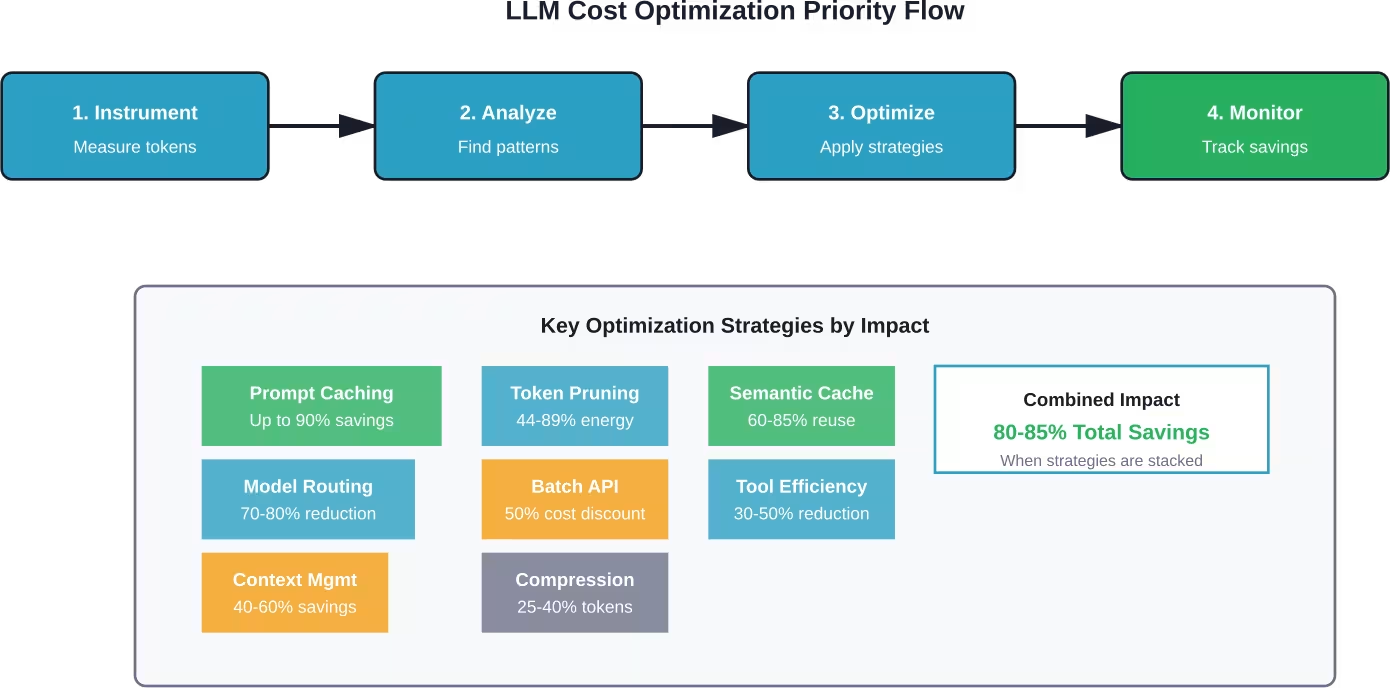
Prompt Caching: The Highest-Impact Quick Win
Prompt caching delivers the single largest cost reduction for most production workloads. The mechanism is straightforward: providers like Anthropic and OpenAI cache the key-value matrices from attention calculations for prompt prefixes. When subsequent requests share that prefix, cached portions cost 90% less.
On Amazon Bedrock, prompt caching reduces inference response latency by up to 85% and input token costs by up to 90%. The math is compelling: a 10,000-token prompt that costs $0.30 per request drops to $0.03 when cached—a $0.27 savings per hit.
But caching effectiveness depends entirely on request patterns. High cache hit rates require stable prompt structures with variable content inserted at predictable positions.
Designing Cache-Friendly Prompts
Cache optimization starts with prompt architecture. Place static content—system instructions, few-shot examples, documentation references—at the beginning. Variable content like user queries and session-specific data goes at the end.
Poor structure:
User query: [VARIABLE]
System instructions: [STATIC 5000 tokens]
Examples: [STATIC 3000 tokens]
Optimized structure:
System instructions: [STATIC 5000 tokens]
Examples: [STATIC 3000 tokens]
User query: [VARIABLE]
The second approach caches 8,000 tokens per request. At typical pricing, a workload with 80% cache hit rate reduces costs by 72% compared to no caching.
Cache eviction policies vary by provider. Anthropic’s cache expires after 5 minutes of inactivity. For sustained workloads, maintaining “warm” caches with periodic requests can be worthwhile if request volume justifies it.
When Caching Pays Off
Not every workload benefits equally from caching. Calculate expected savings:
Break-even cache hit rate = Cache write cost / (Uncached cost – Cached cost)
For prompts under 1,000 tokens, cache overhead often exceeds savings unless hit rates exceed 85-90%. Sweet spots emerge with:
- Large static contexts (documentation, knowledge bases)
- Repeated system instructions across requests
- Few-shot examples in every prompt
- Conversation histories with new messages appended
A documentation chatbot with 15,000-token context and 500-word queries benefits enormously. A creative writing assistant generating unique stories each time? Probably not.
Semantic Caching: Beyond Exact Matches
Traditional caching requires identical inputs. Semantic caching recognizes that “How do I reset my password?” and “What’s the process for password recovery?” deserve the same cached response.
Implementation uses vector embeddings to measure query similarity. Each request generates an embedding (100-300 dimensions typically), which is compared against cached embeddings using cosine similarity or other distance metrics. When similarity exceeds a threshold (commonly 0.85-0.95), the cached response returns instead of invoking the LLM.
Semantic caching operates at a different layer than provider prompt caching. Prompt caching reduces input token costs for cache hits but still invokes the model. Semantic caching avoids the model call entirely, eliminating both input and output costs plus latency.
Building a Semantic Cache Layer
Effective semantic caching requires several components:
- Embedding model: Lightweight and fast (Sentence-BERT, MiniLM)
- Vector database: Redis, Pinecone, Qdrant, or similar for similarity search
- Cache key generation: Combination of embedding similarity and metadata filters
- Similarity threshold tuning: Balance between cache hit rate and response relevance
- TTL policies: Expiration for time-sensitive content
The similarity threshold matters immensely. Too high (0.98+) and cache hit rates drop unnecessarily. Too low (0.80-) and irrelevant cached responses degrade quality. Start at 0.90 and tune based on manual review of borderline cases.
Metadata filtering prevents inappropriate cache hits. A question about “Product A pricing” shouldn’t return cached responses about “Product B pricing” even with high semantic similarity. Tag cached entries with relevant attributes (product, user segment, date range) and require metadata matches alongside semantic similarity.
Hybrid SLM + LLM Routing: Match Models to Tasks
The frontier model fallacy assumes bigger models always perform better. Reality proves more nuanced. Small language models (SLMs) with 7-9 billion parameters handle many production tasks at 10-50x lower cost than 70B+ parameter alternatives.
Research on LLM shepherding shows that even hints comprising 10–30% of the full LLM response improve SLM accuracy significantly, with diminishing returns beyond 60%. This approach can be used in hybrid architectures where SLMs handle most work and LLMs provide targeted assistance when needed.
Hybrid orchestration can route requests based on complexity, with simple tasks potentially flowing to SLMs and complex reasoning escalating to larger models.
Implementing Intelligent Routing
Effective routing requires a classification layer that predicts task complexity before invoking models. Several approaches work:
| Routing Strategy | Complexity | Accuracy | Cost Impact |
|---|---|---|---|
| Rule-based | Low | Moderate | 60-70% reduction |
| Keyword matching | Low | Moderate | 50-65% reduction |
| Classifier model | Medium | High | 70-80% reduction |
| Confidence scoring | High | Very high | 75-85% reduction |
| Cascade with fallback | Medium | Very high | 65-80% reduction |
Rule-based routing proves simplest: “Questions under 20 tokens go to SLM, over 100 tokens to LLM.” This works for clear-cut distinctions but misses nuance.
Classifier models train on historical data labeled with ground truth complexity. Features include query length, vocabulary diversity, presence of specific keywords, and past model performance on similar queries. Lightweight classifiers (100-300M parameters) add minimal latency while improving routing accuracy.
Confidence scoring takes a different approach: always try the SLM first, check confidence scores in the response, and escalate to the LLM only when confidence falls below threshold. This “optimistic routing” minimizes unnecessary LLM calls while maintaining quality.
The Cascade Pattern
Cascading combines routing with validation. Every request starts at the smallest capable model. If that model’s response meets quality thresholds, return it. Otherwise, escalate to the next larger model.
Quality thresholds might include:
- Confidence scores from the model itself
- Format validation (properly structured JSON, complete sentences)
- Length requirements (minimum word count)
- Semantic coherence checks
Research on Pyramid MoA frameworks demonstrates cascade systems matching Oracle baseline accuracy of 68.1% while enabling up to 18.4% compute savings. The router transfers zero-shot to unseen benchmarks, maintaining robustness across different task types.
The trade-off? Latency. Cascading adds the time cost of failed attempts. For latency-sensitive applications, upfront routing with a classifier model performs better than cascading with validation.
Context Management and Compression
Context windows keep expanding—128K, 200K, even 1M tokens—but bigger isn’t always better. Each token in your context costs money on input and influences output generation costs. Bloated contexts burn budgets without improving results.
Effective context management balances information completeness against token economy. The goal: include sufficient context for accurate responses while excluding redundant or irrelevant information.
Context Compression Techniques
Research on sentence-anchored gist compression shows pre-trained LLMs can be fine-tuned to compress contexts by factors of 2x to 8x without significant performance degradation.
Practical compression strategies include:
- Summarization: Condense long documents or conversation histories into summaries
- Extraction: Pull relevant snippets rather than including full documents
- Pruning: Remove redundant information from repeated contexts
- Hierarchical context: Provide high-level summaries with detail available on request
Conversation history represents a common compression target. Instead of sending 50 message pairs (100 messages total), summarize older exchanges and include only recent messages verbatim. This typically reduces context by 60-80% with minimal information loss.
Document retrieval workflows benefit from extraction over inclusion. Rather than stuffing 10 full documentation pages into context (15,000 tokens), extract relevant sections totaling 2,000-3,000 tokens. Retrieval augmented generation (RAG) architectures excel here, using vector similarity to identify pertinent passages.
Sliding Window Contexts
For ongoing conversations or monitoring tasks, sliding windows maintain fixed-size contexts by discarding old information as new information arrives. The window size balances context preservation against cost.
Implementation tracks token counts across context elements:
- System instructions: Fixed allocation (e.g., 1,000 tokens)
- Recent messages: Variable allocation (e.g., last 10 exchanges, ~3,000 tokens)
- Summary of older context: Fixed allocation (e.g., 500 tokens)
- Current query: Variable (user input)
When total context exceeds limits, regenerate the summary to incorporate older recent messages, then discard those messages. This maintains context continuity while capping token consumption.
Token-Efficient Tool Use and Function Calling
LLM function calling enables structured interactions with external systems, but tool definitions consume significant context. A complex API with 20 available functions might require 5,000-8,000 tokens just describing those functions—before any actual work happens.
Token-efficient tool use optimizes both tool definitions and calling patterns to minimize overhead while maintaining functionality.
Optimizing Tool Schemas
Function definitions follow JSON Schema format, which can be verbose. Consider this bloated example:
{
“name”: “get_user_information”,
“description”: “This function retrieves comprehensive user information from the database including personal details, account status, preferences, and history.”,
“parameters”: {
“type”: “object”,
“properties”: {
“user_identifier”: {
“type”: “string”,
“description”: “The unique identifier for the user, which can be either their username or email address”
}
}
}
}
Compressed version:
{
“name”: “get_user”,
“description”: “Get user details by username or email”,
“parameters”: {
“type”: “object”,
“properties”: {
“id”: {“type”: “string”, “description”: “Username/email”}
}
}
}
The compressed version cuts tokens by 60% while preserving functionality. Apply these principles:
- Shorter function names when unambiguous
- Concise descriptions (10-15 words maximum)
- Abbreviated parameter names
- Minimal parameter descriptions
- Remove optional parameters rarely used
Dynamic Tool Provisioning
Instead of providing all available tools in every request, provision tools based on query analysis. A question about “user accounts” loads user management tools; a question about “product inventory” loads inventory tools.
This requires a tool selection layer before the main LLM call:
- Analyze the query with a lightweight classifier
- Map query categories to relevant tool sets
- Include only applicable tools in context
- Process with main LLM
For applications with 50+ available tools, dynamic provisioning reduces tool definition overhead from 15,000 tokens to 2,000-4,000 tokens—an 80% reduction in tool-related context consumption.
Batch Processing for Non-Urgent Workloads
OpenAI’s Batch API and similar offerings from other providers deliver 50% cost discounts for asynchronous processing. The trade-off is latency: batch requests complete within 24 hours rather than seconds.
Batch processing makes sense for:
- Offline analysis and reporting
- Bulk content generation
- Data labeling and annotation
- Nightly summarization jobs
- Model evaluation and testing
It doesn’t work for:
- User-facing chat interfaces
- Real-time decision systems
- Time-sensitive alerts
- Interactive applications
Workload classification determines batch suitability. A content recommendation engine might generate recommendations in batches overnight, then serve them from cache during the day. This hybrid approach captures batch discounts without sacrificing user experience.
Implementing Batch Workflows
Effective batch processing requires workflow orchestration:
- Collection phase: Accumulate requests that can tolerate delayed processing
- Batch submission: Package requests and submit to batch API
- Status monitoring: Track batch progress and handle failures
- Result processing: Retrieve completed results and update systems
- Cache population: Store results for fast retrieval
Batch size optimization matters. Larger batches amortize fixed overhead but increase failure risk and retry costs. Smaller batches complete faster but multiply API calls. Sweet spots typically range from 100-1,000 requests per batch depending on individual request complexity.
Model Selection Strategy: Right-Sizing Intelligence
Model selection represents one of the most impactful cost levers. Pricing varies dramatically across model tiers, yet many applications default to premium models for all tasks.
| Model Class | Parameters | Typical Cost/1M Tokens | Best For |
|---|---|---|---|
| Micro models | 1-3B | $50-100 | Classification, extraction, routing |
| Small models | 7-9B | $100-300 | Simple Q&A, templated generation |
| Medium models | 30-40B | $500-1,000 | Complex reasoning, technical tasks |
| Large models | 70B+ | $2,000-5,000 | Advanced reasoning, creative work |
| Frontier models | 400B+ | $10,000-30,000 | Research, most difficult tasks |
Amazon Nova Micro illustrates this pricing spectrum: $0.035 per million input tokens, roughly 100x cheaper than frontier alternatives. For tasks within its capability range, Nova Micro delivers massive cost advantages.
The strategy: match model capability to task difficulty. Classification tasks don’t need reasoning powerhouses. Simple Q&A over structured data works fine with smaller models. Reserve expensive models for genuinely difficult problems.
Progressive Model Testing
When implementing new features, test progressively from smallest to largest models:
- Start with the smallest model that might work
- Measure quality metrics against requirements
- If quality insufficient, move up one tier
- Repeat until quality requirements met
- Use that model tier in production
This prevents over-provisioning. Teams often assume complex tasks require frontier models, then discover 30B parameter models perform adequately. That assumption costs 10-20x more than testing would reveal.
Monitoring, Alerts, and Cost Governance
Cost optimization isn’t a one-time project—it requires ongoing monitoring and governance. Production systems drift over time as usage patterns evolve and new features launch.
Essential Cost Metrics
Track these metrics daily or weekly:
- Total cost: Overall spend across all LLM operations
- Cost per request: Average cost for individual operations
- Cost by model: Spend breakdown across model tiers
- Cost by feature: Attribution to product capabilities
- Token efficiency ratio: Output tokens / input tokens
- Cache hit rate: Percentage of requests served from cache
- Model routing distribution: Percentage of requests by model tier
Set alerts for anomalies:
- Daily spend exceeds 150% of 7-day moving average
- Cost per request increases more than 50% week-over-week
- Cache hit rate drops below historical baseline
- Single user/feature consumes over 20% of daily budget
Alerts enable rapid response to cost spikes before they accumulate into budget crises.
Cost Allocation and Chargebacks
For organizations with multiple teams or products sharing LLM infrastructure, cost allocation creates accountability. Tag every request with attribution metadata:
- Team or business unit
- Product or feature
- Environment (production, staging, development)
- User segment (free, premium, enterprise)
Generate weekly cost reports showing spend by dimension. Teams that see their consumption patterns make more informed optimization decisions than those operating without visibility.
Chargebacks—actually billing internal teams for their LLM usage—create stronger incentives for efficiency. When cost appears as a line item in team budgets rather than a shared overhead, optimization becomes a priority.
Advanced Optimization: Quantization and Fine-Tuning
Beyond operational optimizations, model-level techniques offer additional cost reduction for self-hosted deployments.
Quantization
Quantization reduces model precision from 16-bit or 32-bit floating point to 8-bit or 4-bit integers. This cuts memory requirements and speeds inference while introducing minimal quality degradation when done carefully.
According to Hugging Face sources, pruning can reduce model size significantly (often 80-90%) with minimal performance degradation when done carefully. At 50% sparsity, WiSparse preserves 97% of Llama3.1’s dense model performance.
For self-hosted deployments, quantization can reduce memory requirements significantly. Model-specific memory requirements depend on parameter count and precision level.—enabling deployment on cheaper hardware or serving more requests per GPU.
Trade-offs matter. Aggressive quantization (2-bit, 1-bit) degrades quality noticeably. Conservative quantization (8-bit) preserves quality but reduces savings. Most production deployments target 4-bit as the sweet spot.
Fine-Tuning for Efficiency
Fine-tuned models can be smaller and cheaper while maintaining performance for specific domains. A general-purpose 70B parameter model might be replaced with a fine-tuned 7B model for narrow applications.
Fine-tuning requires:
- High-quality training data (hundreds to thousands of examples)
- Compute resources for training (GPUs, hours to days)
- Evaluation infrastructure to validate quality
- Ongoing maintenance as requirements evolve
The economics favor fine-tuning when:
- Request volume is very high (millions per month)
- Task requirements are stable
- Performance quality can be rigorously measured
- Infrastructure exists for model hosting
For API-based workflows, fine-tuning costs exceed savings until monthly request volumes reach hundreds of thousands or millions of calls.
The 2026 Cost Optimization Stack
Effective LLM cost management in 2026 combines multiple strategies into a coherent architecture. No single technique solves all problems—the best results come from stacking complementary approaches.
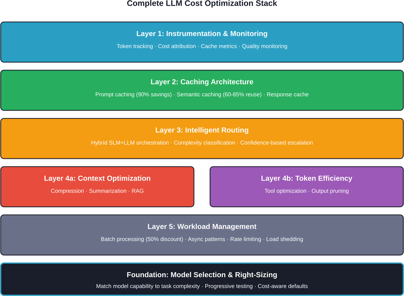
A production-grade optimization stack includes:
- Foundation layer: Model selection strategy ensures tasks use appropriately-sized models by default.
- Caching layer: Both prompt caching and semantic caching intercept redundant work before it reaches models.
- Routing layer: Intelligent orchestration directs requests to the most cost-effective model capable of handling them.
- Optimization layer: Context compression, token efficiency, and output management minimize waste in requests that reach models.
- Workload layer: Batch processing and async patterns capture discounts for non-urgent work.
- Governance layer: Monitoring, attribution, and alerts maintain optimizations over time and prevent cost drift.
Each layer contributes independently, but combined effects multiply. A system using all six layers achieves 80-85% cost reduction compared to naive implementations—transforming a $216,000 annual spend into $30,000-$40,000 while maintaining or improving quality.

Reduce LLM Costs Early – Fix the Setup Before Scaling
Most cost issues in LLM projects come from how systems are set up, not just how they are used. Inefficient data pipelines, oversized models, and unoptimized prompts can quietly drive costs up long before scaling begins. AI Superior works across the full lifecycle – from data preparation and model design to training, fine-tuning, and deployment – helping teams remove these inefficiencies early instead of reacting later.
The focus is on making models usable in production without unnecessary overhead, whether that means adjusting model size, refining workflows, or rethinking when to rely on external APIs versus custom setups. This becomes critical once usage grows, where small inefficiencies turn into real spend. If you are trying to cut LLM costs in a practical way, it is worth reviewing your setup before scaling further. Reach out to AI Superior to identify where costs can actually be reduced.
Common Pitfalls to Avoid
Cost optimization attempts often fail due to predictable mistakes. Avoiding these accelerates success.
Optimizing Without Measuring
The most common failure mode: implementing optimizations without instrumenting their impact. Teams deploy caching, assume it works, and miss that cache hit rates hover around 20% instead of the expected 80%.
Measurement must precede optimization. Otherwise, efforts focus on areas with minimal impact while high-cost drivers remain unaddressed.
Over-Optimizing Latency
Latency and cost trade off. Aggressive caching reduces costs but adds cache lookup latency. Cascading routing saves money but increases failed-attempt delays. Batch processing delivers massive discounts but eliminates real-time response.
Not every millisecond matters equally. A customer-facing chat interface needs sub-second response times. An overnight report generator can tolerate minutes. Match optimization strategies to actual latency requirements rather than optimizing everything for speed.
Neglecting Quality Monitoring
Cost optimization shouldn’t degrade output quality, but aggressive techniques sometimes do. Overly aggressive compression loses critical context. Semantic caching with overly loose similarity thresholds may return responses that don’t match query intent closely. Routing to smaller models reduces capability.
Quality monitoring must run alongside cost monitoring. Track metrics like:
- User satisfaction scores
- Task completion rates
- Error rates and retries
- Manual review of sample outputs
When cost optimization hurts quality, the optimization fails regardless of savings achieved.
Ignoring Hidden Costs
Token costs represent the obvious expense, but hidden costs accumulate:
- Engineering time building and maintaining optimization infrastructure
- Infrastructure costs for caching layers and monitoring systems
- Increased complexity and debugging difficulty
- Opportunity cost of team attention on cost rather than features
Calculate true ROI including these factors. A caching system that saves $500 monthly but requires $300 in infrastructure and 20 engineering hours to maintain delivers questionable value.
Frequently Asked Questions
What’s the single highest-impact LLM cost optimization for most applications?
Prompt caching typically delivers the largest immediate impact for applications with stable prompt structures. When applicable, caching can reduce input token costs by 90% and latency by 85%. Implementation is straightforward—restructure prompts to place static content first—and doesn’t require complex infrastructure. Most production applications with documentation, examples, or repeated instructions in prompts benefit significantly.
How do I know if my cache hit rate is good enough?
Cache hit rates above 60% can provide meaningful cost savings with prompt caching. Semantic caching needs higher rates—typically 70-80%—because implementation costs more. Calculate expected savings: (hit_rate × cache_savings) – cache_costs. If that number exceeds 40-50% net reduction, caching pays off. Monitor hit rates weekly; drops indicate prompt structure changes or query pattern shifts that need addressing.
Should I use SLMs or LLMs for classification tasks?
Classification tasks almost always benefit from smaller models. Research shows 7-9B parameter models achieve 85-95% of large model accuracy on classification while costing 10-50x less. Test your specific classification task: collect 100-200 labeled examples, evaluate both small and large models, and compare accuracy. Unless the accuracy gap exceeds 5-10 percentage points, choose the smaller model.
When does model fine-tuning pay off versus using larger models?
Fine-tuning becomes economical when monthly request volume exceeds several hundred thousand calls and task requirements remain stable. Training costs range from $500-5,000 depending on model size and data volume. If a fine-tuned 7B model replaces a 70B API at 30x lower inference cost, break-even occurs around 300,000-500,000 requests. Below that volume, optimization techniques like caching and routing deliver better ROI.
How much context compression is safe without losing quality?
Safe compression ratios depend heavily on content type. Conversation history compresses 60-80% with summarization while maintaining coherent dialogue. Technical documentation typically compresses 40-60% through extraction without information loss. Creative or nuanced content compresses less—maybe 30-40%. Always A/B test: process identical queries with full and compressed contexts, compare outputs, and measure quality differences before deploying compression.
What’s the minimum viable instrumentation for LLM cost tracking?
At minimum, log these six fields per request: timestamp, model_name, input_tokens, output_tokens, calculated_cost, and one attribution field (user_id or feature_name). Store in any database supporting aggregation queries—even a simple PostgreSQL table works. This enables daily cost monitoring and identifies high-spend areas. Add more fields (latency, cache_hit, quality_score) as needs emerge, but start with these basics.
How do I convince leadership to invest in LLM cost optimization?
Present cost projections with and without optimization. Show current monthly spend, multiply by 12 for annual cost, then calculate optimized annual cost using conservative savings estimates (50-60% rather than 80%). The delta—often $100,000+ for production applications—justifies engineering investment. Include ROI calculation: (Annual_Savings – Implementation_Cost) / Implementation_Cost. ROI above 300% makes the case compelling.
Conclusion: From Cost Center to Competitive Advantage
LLM costs don’t have to spiral out of control. The strategies outlined here—prompt caching, intelligent routing, context optimization, and systematic instrumentation—consistently reduce production costs by 70-85% while maintaining or improving quality.
But this isn’t just about saving money. Organizations that master cost-efficient LLM operations gain strategic advantages. Lower unit economics enable serving more users, experimenting with new features, and delivering AI capabilities competitors find economically unviable.
The key insight: treat token consumption as a first-class engineering concern from day one. Instrument early, optimize systematically, and monitor continuously. The techniques that work in 2026—caching, routing, compression—will evolve, but the discipline of cost-aware LLM engineering will remain essential.
Start with measurement. Pick one high-traffic feature, instrument its token consumption, and analyze patterns. That visibility unlocks optimization opportunities worth 10-100x the instrumentation effort. Then apply targeted strategies where data shows they’ll have the most impact.
The organizations winning with LLM technology in 2026 aren’t just those with the best models—they’re those who’ve mastered the economics of putting models into production efficiently.